Machine Learning 3

Clustering

I. Defining Clusters

A cluster is a group of similar examples. Define cluster $k$ by a prototype $\mu_k$. $r_{nk}$ is an indicator variable, $r_{nk} \in$ {0, 1}, 1 means example $n$ is in cluster $k$; 0 means example $n$ is not in cluster $k$. The restriction is that every example must be in one cluster, $r$ is going to be a matrix where the rows of the matrix are going to sum to 1.

Compute the average of all the examples in that cluster. For every example, if it is in the cluster (i.e. $r_{nk}=1$), sum it and divide by the number of examples in that cluster.

\[\mu_k = \frac{1}{\sum^N_{n=1}r_{nk}}\sum^N_{n=1}r_{nk}\mathbf{x}_n\]

II. Objective

Maximize the similarity of every cluster.

Distortion measure: for every example in that cluster, how far is that example from the mean of the cluster.

\[J = \sum^N_{n=1}\sum^K_{k=1}r_{nk}||\mathbf{x}_n-\mu_k||^2\]

There are two parameters: cluster means $\mu_k$ and the assignment of examples to clusters $r_{nk}$. We aim to select $\mu$ and $r$ such that they minimize $J$.

Learning procedure: each update reduces the value of $J$ (can’t be negative). Therefore it will converge. Note: $J$ is non-convex. Therefore, resulting value may not be the best. initial value matter! If I have a good initialization then I’m going to get a better solution. This is called k-means.

III. K-means

(1) Given data \(\{(\mathbf{x}_i)\}^N_{i=1}, \mathbf{x}_i \in \Re ^N\).

(2) Randomly initialize $\mu_k$.

(3) Iteratively update until convergence:

​ (3.1) assign every point to the closest $\mu_k$.

​ (3.2) recompute means $\mu_k$.

Limitations

• You have to pick $k$, k-means (Minimize distortion $J$) doesn’t tell you what $k$ is.

  Solution: Hierarchical clustering

• highly sensitive to outliers.

  Solution: k-medoids

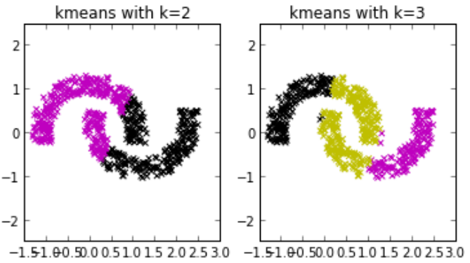
• Works poorly on non-convex clusters.

  Solution: Spectral Clustering

  

• Assumes spherical, equally likely clusters.

  Solution: Spectral Clustering

• Hard assignment of example to clusters.

  Solution: Probabilistic clustering

IV. Components of clustering

Distance Measures

K-means is using Euclidean distance $d(x_i, x_j) = \sqrt{\sum^D_{d=1}(x_{i,d}-x_{j,d})^2}$. It is invariant to rotation and translation of features but not to scaling.

Loss Function

Caveat: Some clustering is convex but requires assumptions.

Evaluation

We cannot compare different clusterings by evaluating a loss function without labels. We need a small set of labeled examples to validate different clustering algorithms.

What metrics to use? - cannot use accuracy

(1) Purity: Assign each cluster to the class which is most frequent in the cluster. Drawback: high purity when many clusters. So purity is only useful if you are comparing clusterings that use the same number of clusters.

(2) Normalized mutual information NMI: How much do we learn about the labels when we are told the clusters?

\[NMI(Y,C)=\frac{2 \times MI(Y;C)}{H(Y) + H(C)}\]

where $MI$ is mutual information, and $H$ is entropy.

Algorithm

Hierarchical Clustering

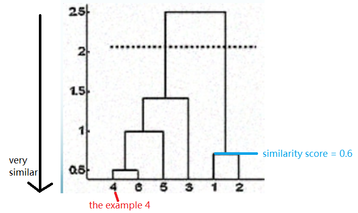
Don’t choose $k$. Move from flat clusters to hierarchical clusters. Define an organization over the dataset without specifying clusters.

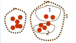
Horizontal line cuts tree into clusters based on post-hoc decision of $k$. Below is the dendrogram:

Divisive (Top Down) Clustering vs. Agglomerative (Bottom Up) Clustering

• Agglomerative cluster is usually faster, because it only considers “local” clusters in a merge.

• Divisive may be more sensitive to global data structure. We have access to all the data when making our first split. The advantage of the top down method is you could look at the global properties of the data and don’t just make local decisions, but that might be more expensive.

  You can get more balanced tree by going top down. You can make the criteria of top down.

K-medoids

Instead of mean, K-medoids picks the median (the example closest to the mean) of the cluster to serve as the cluster prototype.

Spectral Clustering

Spectral Clustering is a partitional clustering but not based on spherical clusters. Construct a graph G from the data: ● Vertices - examples ● Edges - weighted similarity between examples

• Goal of clustering: Partition the vertices of the graph.
• Loss function: measured by a cut of the graph.
  • Minimize Cut (mincut): the weight of the edges “cut” (sum of all those edges) by partitioning vertices into different clusters.
  • Requires normalization to force meaningful cuts and ensure clusters are balanced.
  • Minimizing normalized cut is NP-hard.
  • Spectral clustering is a relaxation that can be solved optimally.

Probabilistic Clustering

Clusters are probability distributions. Membership in a cluster is probabilistic, no hard assignments.

• Generative process
  • Select a cluster (a Gaussian distribution)
  • Generate an example by sampling point from the Gaussian

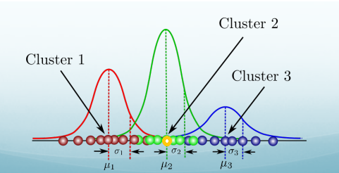
In this case, the yellow point is much more likely come from cluster 2 than any other clusters, but cluster 1 and cluster 3 does give it a probability. So even it’s peaked at cluster 2. It doesn’t have a zero probability belonging to the other clusters.

V. Gaussian Mixtures

$z_k$: $z_k \in {0,1}$ and $\sum_k z_k = 1$. If assign to Gaussian k or not. $P(z_k=1) = \pi_k$.

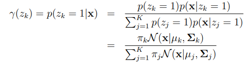
$\mathcal{N}(\mathbf{x}\mid\mu_k, \Sigma_k)$: The probability of Gaussian distribution $k$ generating an example $\mathbf{x}$.

$\gamma(z_{nk})$: the responsibility for cluster $k$ generating point $n$.

$N_k$: the number of points in cluster $k$, or the total responsibility of $k$ for the data.

$\pi_k$: is called the mixture coefficient. It indicates how likely each Gaussian is to generate an example.

$\mu_k$: the mean of cluster $k$.

$\Sigma_k$: the co-variance matrix of cluster $k$.

Maximum Likelihood Updates

• Now that we have a probabilistic model, we can write the likelihood of our data given our model parameters $\pi$, $\mu$ and $\Sigma$.

\[P(\mathbf{X\mid \pi,\mu,\Sigma})=\prod^N_{n=1} \sum^K_{k=1} \pi_k \mathcal{N}(\mathbf{x}_n\mid \mu_k, \Sigma_k)\]

How should we set our model parameters? Let’s use maximum likelihood! First, we write the log-likelihood function:

\[\log P(\mathbf{X\mid \pi,\mu,\Sigma})=\sum^N_{n=1} \log \{ \sum^K_{k=1} \pi_k \mathcal{N}(\mathbf{x}_n\mid \mu_k, \Sigma_k) \}\]

• Let’s begin by taking the derivative with respect to $\mu_k$, $\Sigma_k$ and $\pi_k$, and set the derivative equal to 0 respectively.
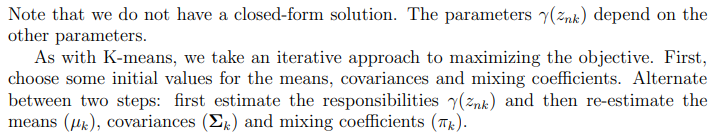
• Finally, we solve $\mu_k$, $\Sigma_k$ and $\pi_k$ respectively. We get:

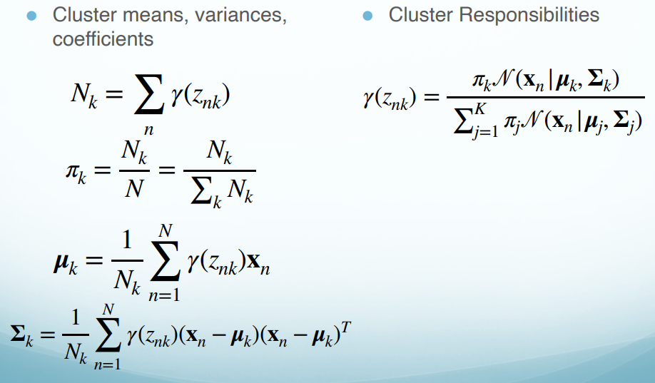
This means that the responsibility for the $k$th Gaussian component is the average responsibility that component takes for explaining the data.

Maximizing Objective

Problems with GMMs

(1) Mode collapse: When a single data point is isolated and becomes its own Gaussian.

(2) Very non-convex likelihood: may end up in a local minimum.

(3) Requires more iterations to converge than K-Means. Plus, each iteration is more computationally expensive.

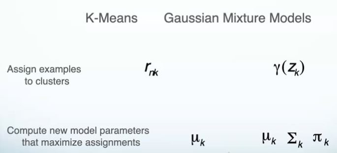
K-means vs. GMMs

Expectation-Maximization Algorithm (EM Algorithm)

A general technique for maximizing likelihood when you have latent variables. EM allows us to write objectives without seeing these variables.

• Expectation step is new! Pretend we see the latent variables.
• Maximization step is familiar. Find the best parameters given the observations.

Exact Inference In Graphical Model

Chain Graphical Model

\[p(x)=\frac{1}{Z} \uppsi_{1,2}(x_1,x_2) \uppsi_{2,3}(x_2,x_3) ... \uppsi_{N-1,N}(x_{N-1},x_N)\]

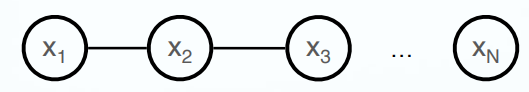
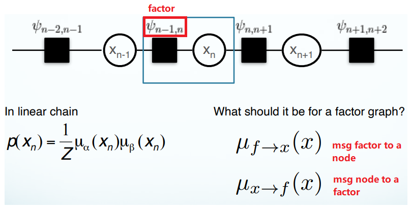
$\frac{1}{Z}$ is normalizer. $\uppsi$ is potential function.

How do I get the probability of a state $p(x_n)$. I have the joint probability of the whole thing. Sum over all of the states they don’t see (i.e. all of possible configurations of the others), that’s marginalization. This naive way takes O($2^N$), because for each x, we have two cases 0 or 1, and we multiply every two cases. Thus, 2 $\times$ 2 $\times$ 2 $\times$ 2 … 

\[p(x_n)=\sum_{x_1}\sum_{x_2}...\sum_{x_{n-1}}\sum_{x_{n+1}}...\sum_{x_N}p(x)\]

By rearranging the term and pushing the $\sum$ in, we get

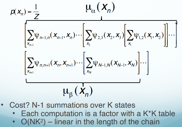
K states: How many possible values of $x$. Cost: For every $x$, we calculate all possible combinations of $K$ states, that is $K^2$ combinations. After, we save the result and use it directly in the following calculations. For example,

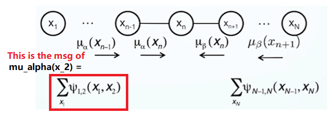
\[\mu_\alpha(x_2)=\sum_{x_1}\uppsi_{1,2}(x_1, x_2) \longrightarrow K^2 \\ \mu_\alpha(x_3)=\sum_{x_2}\uppsi_{2,3}(x_2, x_3)\mu_\alpha(x_2) \longrightarrow K^2\]

We only need to calculate $K^2$ ($N-1$) times. Thus, the time complex is O($NK^2$).

Therefore, the marginal probability of $x_n$:

\[p(x_n)=\frac{1}{Z}\mu_{\alpha}(x_n)\mu_{\beta}(x_n)\]

Each factor ($\mu_{\alpha}(x_n)$, $\mu_{\beta}(x_n)$) depends only on one side of the chain.

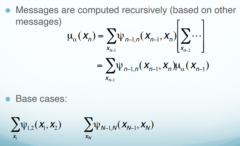
Messages

Calculating the Message

Normalization Constant

$Z$ is sum over all states (i.e. all possible values of $x_n$), which is O(K), cuz we only have $K$ states here. For example, $Z = \mu_{\alpha}(x_3=T)\mu_{\beta}(x_3=T) + \mu_{\alpha}(x_3=F)\mu_{\beta}(x_3=F)$. There is linear # of messages, so the whole algorithm is linear. O($NK^2$) is not only for solving the marginalization for one node $p(x_n)$, but the cost for solving all the marginalizations for everything in the graph.

Exact Inference

Inference is NP-Hard, cuz no efficient algorithm for arbitrary graphical models.

Goal:

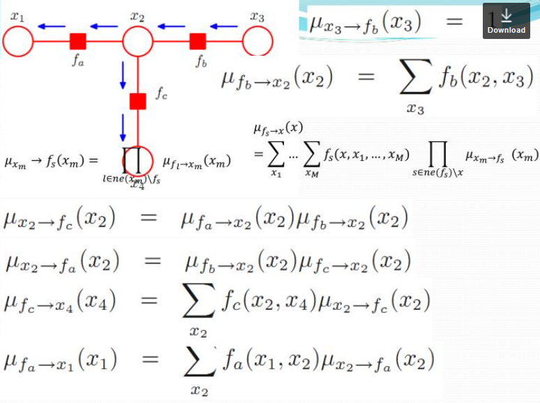
\[p(x) = \prod_{s\in ne(x)} \sum_{X_s}F_s(x, X_s)\]

A product of all the factors coming into this node. $F$ is a factor, $s$ is an index of factors (eg. there are 2 factors coming into the node $x_n$), $ne(x)$ is all the neighboring factors for the node $x$. For the potential function $\uppsi_{n-1}$, where the possible values that can take, it can be $x_{n-1}$ and $x_n$ both. We should sum over all of the possible cases of $ x_{n-1}$ and pass this message.

\[\mu_{f\rightarrow x}(x)=\sum_{X_s}F_s(x,X_s)\]

where $X_s$ is all the other nodes that has a role in the factor. If $f=\uppsi_{n-1,n}$, then $X_s=x_{n-1}$. Here we have $x$ and any other nodes connected to the factor $\uppsi_{n-1,n}$, that is $x_{n-1}$ in this case. Sum over all possible combinations of those nodes.

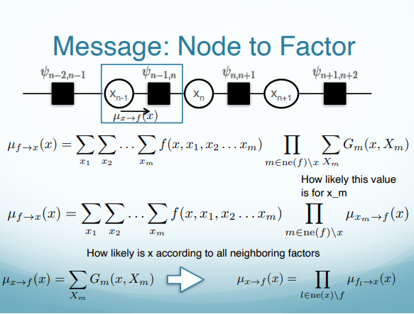
$f$ is a scoring function that assigns a score to different combinations of all the nodes I am attached to (in this case, $x_n$). When you compute the factor multiply by how likely each one of those assignments is according things further down to the chain. For example, when I marginalize $f=\uppsi_{n-1,n}$ over $x_{n-1}$ inside the factor $f(x,x_1,x_2,…,x_n)$, I need to consider whether or not $x_{n-1}$ is likely to be true or false and multiply this. $\mu_{x\rightarrow f}(x)$ is going to say what is the likelihood that I have according to everything further down the chain.

\[\mu_{x\rightarrow f}=\prod_{l\in ne(x)\backslash f} \mu_{f_l \rightarrow x}(x)\]

The message a node sends to a factor = a product of all messages it got from all its neighboring factors.

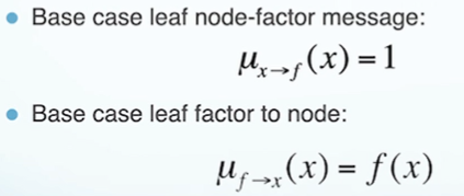
Base cases

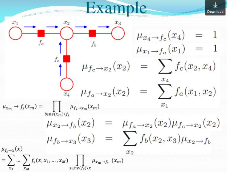
Sum Product Algorithm

(1) reference

(2)

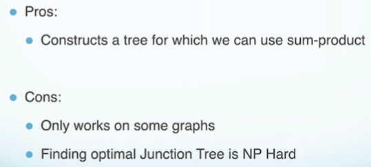
Junction tree

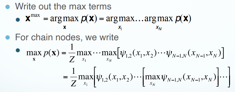
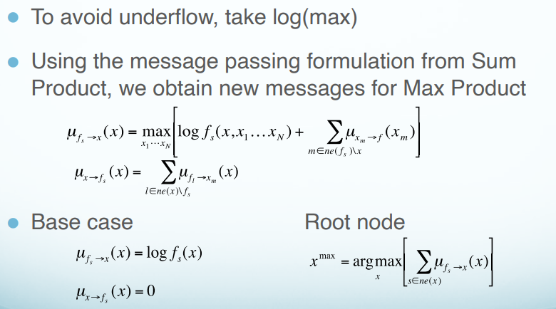
Max Product Algorithm

Max Product Algorithm computes the configuration of the graph that gives the highest global probability.

• We can’t pass messages back as before.
  • There may be multiple configurations that have max value for $p(x)$. Need to distinguish between these configurations.
• Solution: keep track of which states correspond to the same max configuration.

Approximate Inference

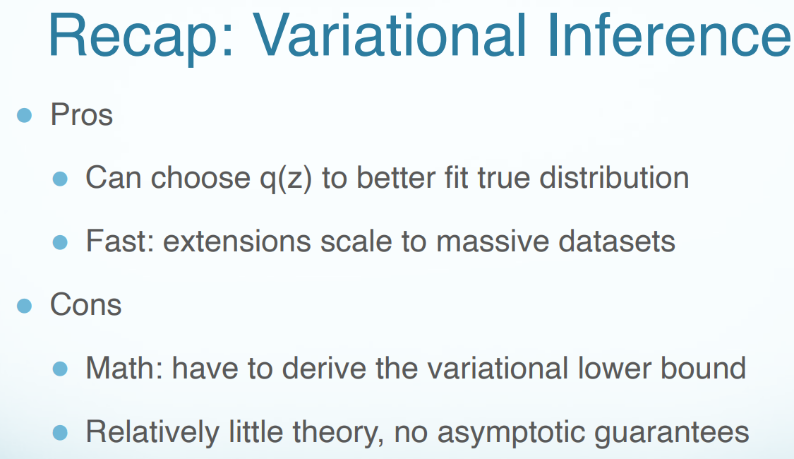
variational Inference

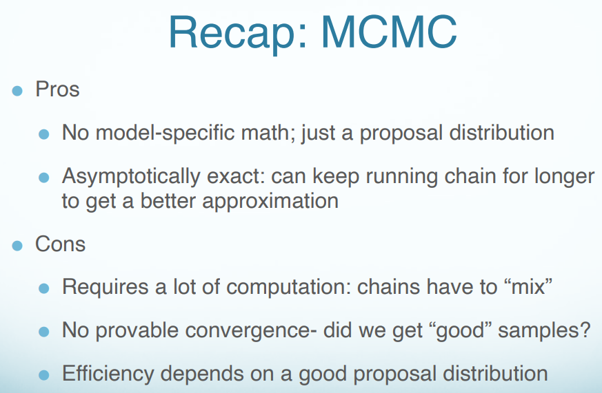
MCMC

Structured Prediction

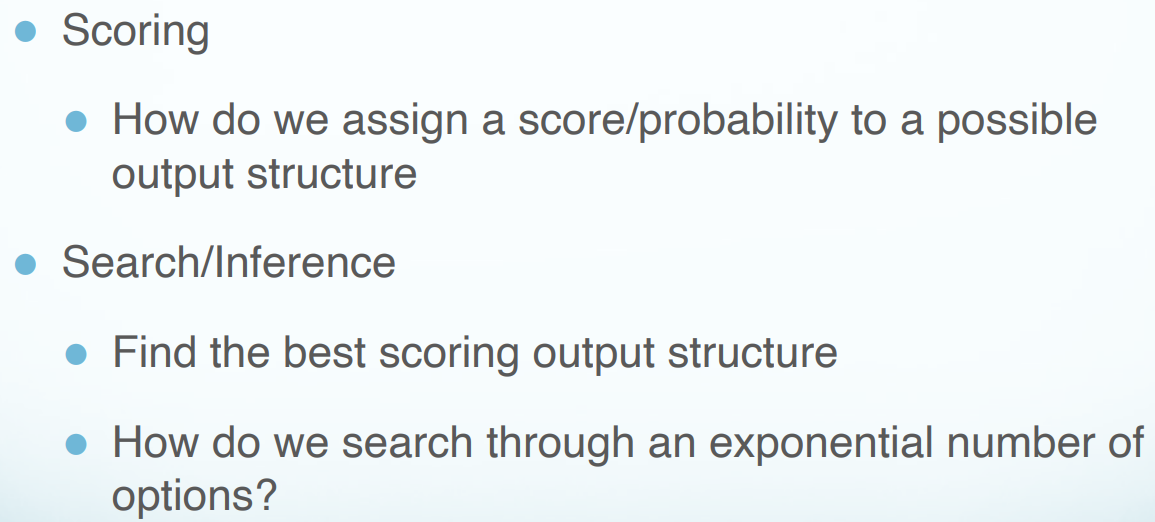
Structured Prediction Challenges

Hidden Markov Model (HMM)

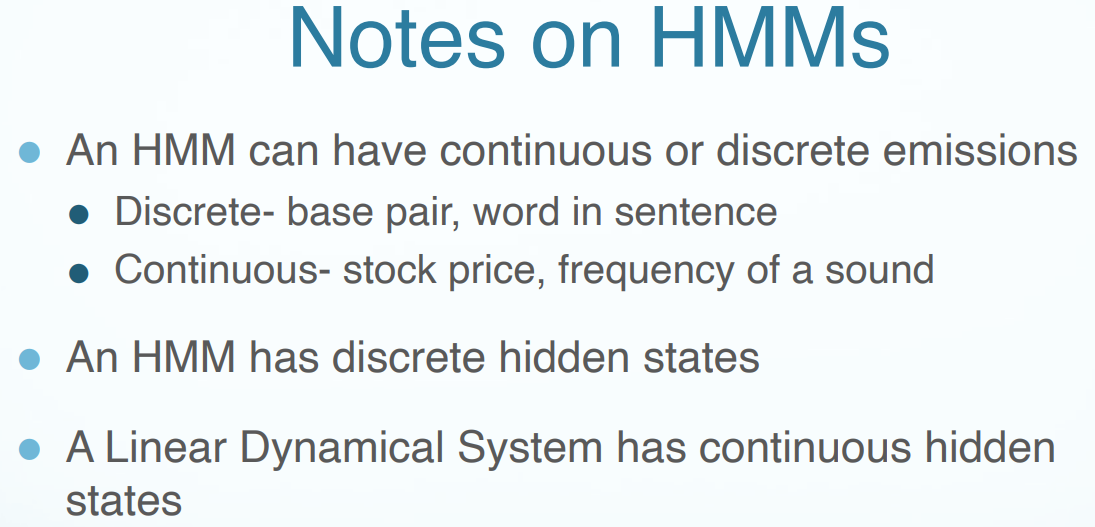
An HMM is a directed graphical model.

Conditional Random Fields (CRF)

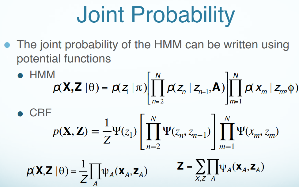
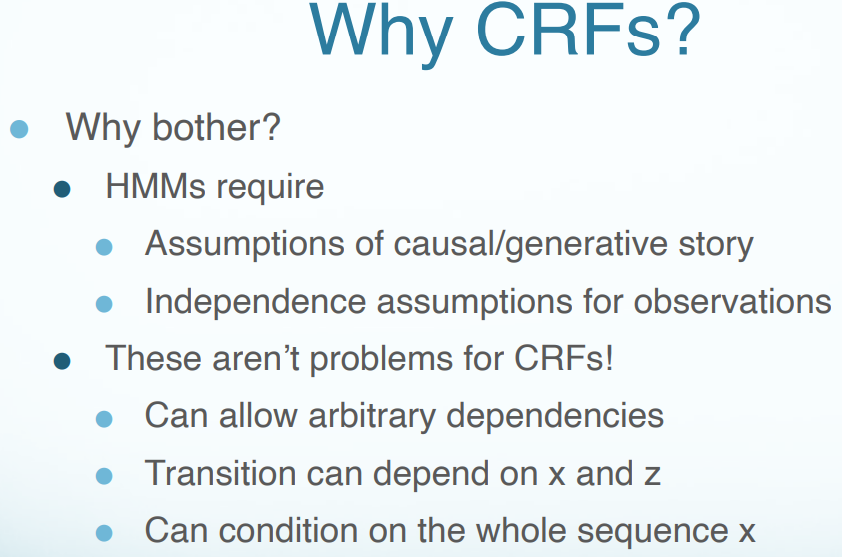
HMMs vs. CRFs

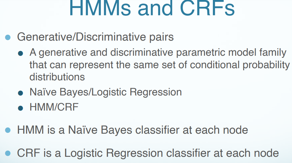
To briefly state the difference between generative models and discriminative models, I would say a generative model concerns the specification of the joint probability $p(x,y)$, and a discriminative model that of the conditional probability $p(y \mid x)$.