Perceptron
We have talked about [ref] [ref2]
| Linear Regression | square Loss | MSE = $\frac{1}{n}\sum^n_{i=1} (y-\hat{y})^2$, where $y$ is the actual value, $\hat{y}$ is the predicted value. |
| Logistic Regression | Log Loss | $L(w) = \sum_{i=1}^{n}-y\text{log}(y’)-(1-y)\text{log}(1-y’)$, where $y$ is the actual value, $y’$ is the predicted value. |
| SVM | Hinge Loss | Loss = $max(0,1-y_i[w^T x_i + b])$, where $y$ is the actual value, $y’$ is the predicted value. |
| AdaBoost | Exponential Loss | $\sum^{n}_{i=1}e^{-y_ih(x_i)}$, where $y_i$ is the actual value, $h(x_i)$ is the predicted value. |
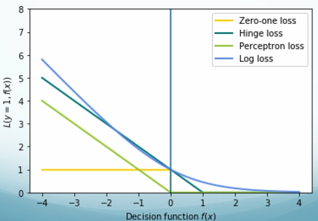
| 0/1 Loss | Wrong: loss of 1; Correct: loss of 0, doesn’t really matter how big mistake you made. |
Perceptron Loss
$L_w(y) = \sum_i^Nmax(0, -y_i(w\cdot x_i))$.
Calculate the gradient of our loss function:
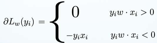
We are only updating the parameters when we are wrong. Update rule:
$w^{i+1} = w^i + \eta \partial L_w(y_i)$
$w^{i+1} = w^i + \eta (y_i - \hat{y}_i)x_i$, where $\hat{y}_i$ = sign($w \cdot x_i$)
$w^{i+1} = w^i + \eta y_i x_i$
Set $\eta$ = 1. If mistake on a positive example $w^{i+1} = w^i + x_i$. If mistake on a negative example $w^{i+1} = w^i - x_i$.
Summary: Perceptron is a linear function. It is a minimization of perceptron loss with a linear hypothesis class. It is a generalized linear model. We are approximating 0/1 loss and we are fitting it using stochastic gradient descent.
For perceptron learning, Bach size ↑, closer to regular gradient descent, noisy ↑, oscillation ↑.
Converge
Will the Perceptron algorithm converge? (i.e. Will it stop making updates?; i.e. Will it stop making mistakes? )
- Yes! The Perceptron is guaranteed to converge on linearly separable data. The Perceptron: converges → updates stop → makes a finite number of mistakes. If the data are linearly separable, the Perceptron will make a finite number of mistakes.
- Data not linearly separable then will not converge.
Smooth Oscillating Behavior of Perceptron Out
Solution: take the best model over time. A model that was good on many examples should be trusted more than the latest model.
Two practical ways:
(1) Voting: Save all the $\mathbf{w}$’s along the way and predict by voting.
(2) Averaging: Take the average of $\mathbf{w}$.
Online Learning
Online learning doesn’t make assumption about the data, doesn’t make assumption about the distribution of the data, and doesn’t make assumption about consistent hypotheses. It operates in the online way. Model learning interacts with a data stream or a human. Predictions needed after each example. It has to keep making predictions and it’s keep getting feedback. Do your best every time we ask you to make prediction and then use that information to do your best the next time.
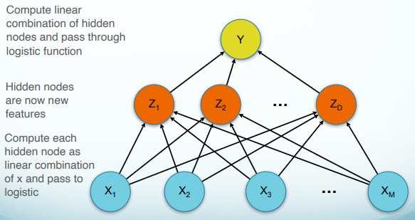
Neural Networks
Multilayer Perceptron is the foundation of neural networks. The power of the network depends on its structure. General result independent of activation functions (assuming non-linear activations).
Network Terminology
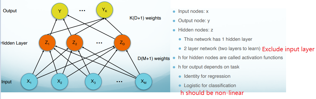
Activation Function
The activation function should:
(1) Ensures not linearity.
(2) Ensure gradients remain large through the hidden unit.
(3) Be differentiable.
Network Structure
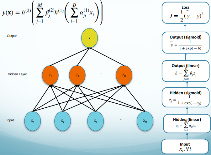
Forward Propagation
Training Objective
-
Classification Objective:
Define an error function and minimize
$E(\mathbf{w}) = \sum_{i=1}^{n}-y_i\text{ln}(y_i’)-(1-y_i)\text{ln}(1-y_i’)$ (= logistic regression)
-
Regression Objective:
We use the sum of squares error:
$E(w) = \frac{1}{2}\sum^n_{i=1} (y-\hat{y})^2$
If we assume a Gaussian model for $y$, the error function arises from maximizing the likelihood function. (= linear regression)
Backpropagation
Gradient based optimization NOT guaranteed to find global optimum.
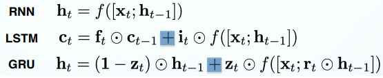
Recurrent Neural Networks (RNNs)
Traditional neural network could not use previous information to predict the future information. Recurrent neural networks address this issue. They are networks with loops in them, allowing information to persist.
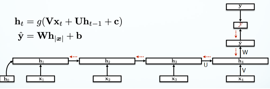
RNN Language Models
RNNs never forget.
Algorithm: Sample a sequence from the probability distribution defined by the RNN. Train the RNN to minimize cross entropy (aka Maximum likelihood estimation).
Vanishing Gradients
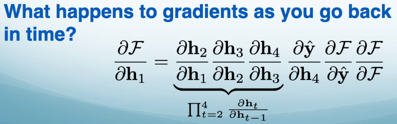
In practice, in $\Pi_{t=2}^4 \frac{\partial h_t}{\partial h_{t-1}}$, $t$ goes to $n$. $\frac{\partial h_t}{\partial h_{t-1}}$ are very small, multiplying lots of small numbers together gives you zero. That’s called vanishing gradient. This means that long-range dependencies are difficult to learn (although in theory they are learnable).
Alternative RNNs
Solutions for vanishing gradients.
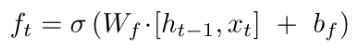
Long short-term memories (LSTMs)
-
Forget gate ($f_t$): decides what information we’re going to throw away from the cell state. It looks at $h_{t−1}$and $x_t$, and outputs a number between $0$ and $1$ for each number in the cell state $C_{t-1}$. (red part)
-
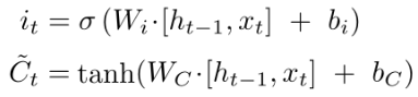
Input gate ($i_t$): decides how much to update each state value.
tanh: creates a vector of new candidate values.
(blue part)
-
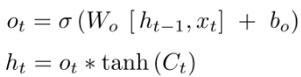
Output gate ($o_t$): decides what parts of the cell state we’re going to output.
tanh: pushes the values to be between $−1$ and $1$.
(orange part)
Summary:

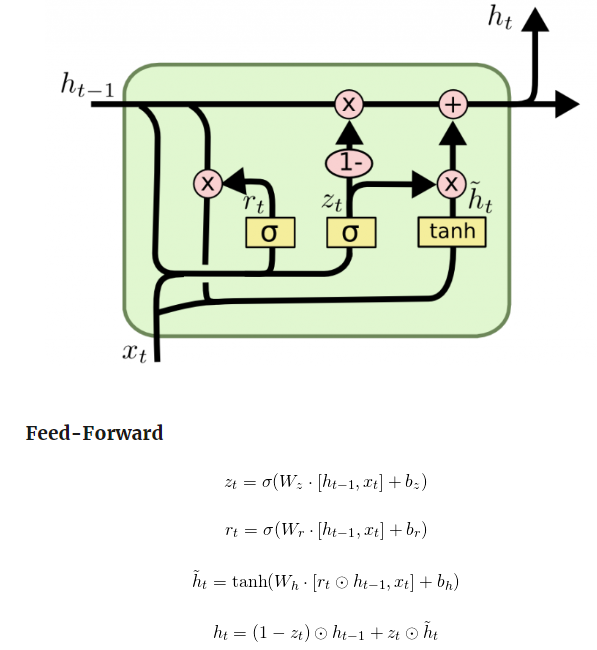
Gated Recurrent Unites (GRUs)
LSTMs have lots of parameters. It’s slow. GRUs are faster. It uses coupled forget and input gates. Instead of separately deciding what to forget and what we should add new information to, we make those decisions together. We only forget when we’re going to input something in its place. We only input new values to the state when we forget something older.
Summary
Better gradient propagation is possible when you use additive rather than multiplicative.
Seq2Seq and Attention
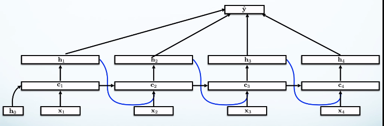
Pooling
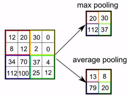
Rather than use $h_4$ to do the prediction, take the average of all the edges.
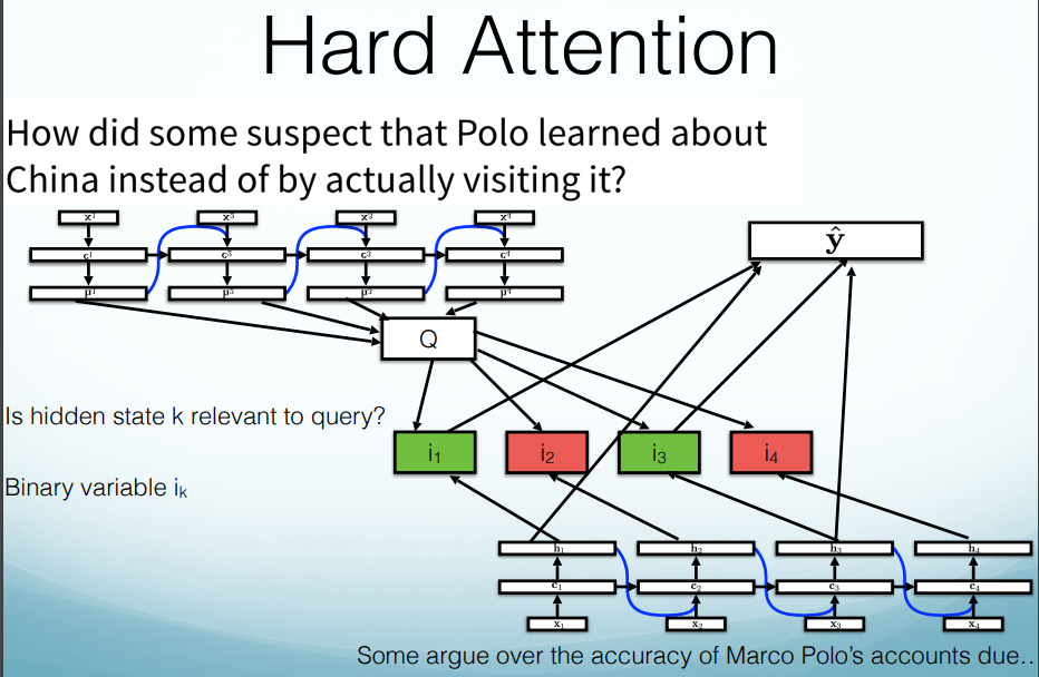
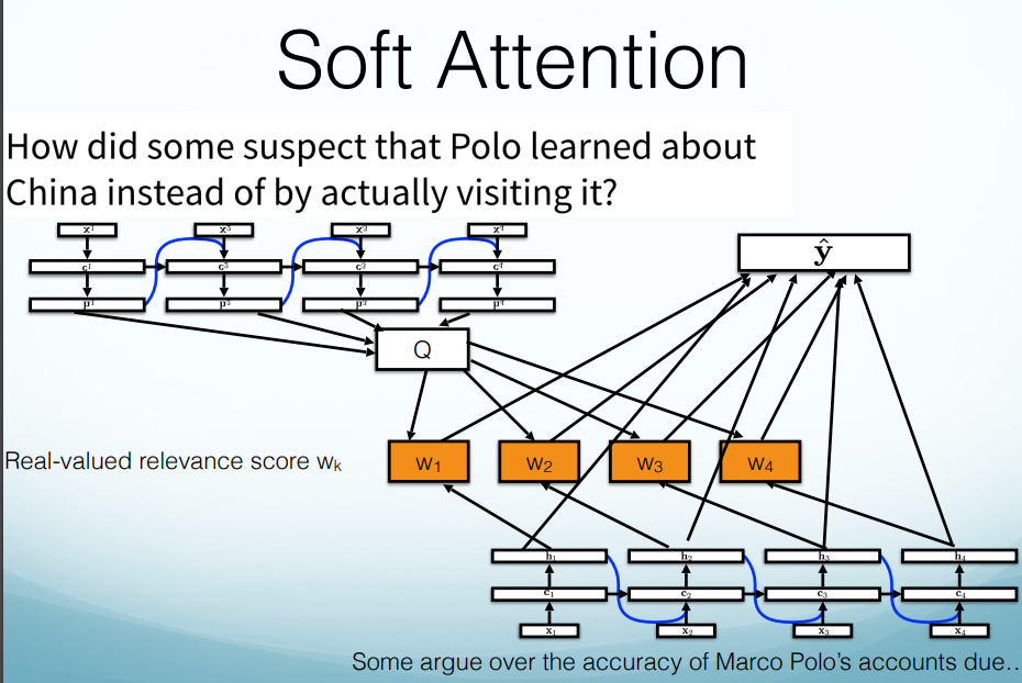
Hard Attention vs. Soft Attention
-
Hard Attention:
(1) First, learn a query representation.
(2) Then pick which pieces of the sequence to include, then answer query based on those pieces.
pros: fast, prediction only uses important pieces.
cons: Non-differentiable (i.e. the network can either pay “attention” or not, with no in between), hard to train these models.
-
Soft Attention:
(1) First, learn a query representation.
(2) Then score each piece of the input to decide how relevant it is to the query. Predict using weighted average of all hidden states.
pros: Differentiable: can train “is it relevant” model with backprop.
con: Slow: score and sum over all hidden states.
Transformer
Each layer looks at all tokens in both directions. No fixed direction.
Pro: (1) Distance is no longer a factor. Can attend to any token in the sequence, no matter the distance.
(2) No forward/back propagation through sequence, now only through layers.
(3) Much easier to parallelize.