Regression
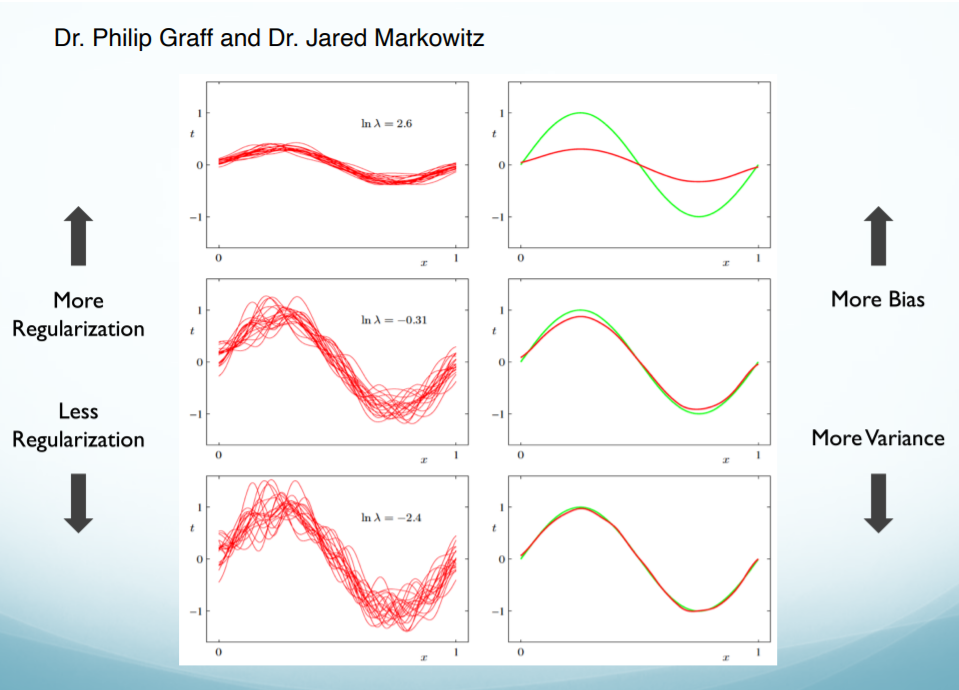
Regularization
Regularization refers to techniques that are used to calibrate machine learning models in order to minimize the adjusted loss function and prevent overfitting or underfitting.
L2 Ridge Regression vs. L1 Lasso Regression vs. Ordinary least squares linear regression
When would you want to use (i) Ridge regression, (ii) Lasso regression, (iii) Ordinary least squares linear regression?
(i) When we have many predictors, we want to shrink the coefficients of the low variance components of the input vector $\mathbf{x}$. Same as weight decay, the $L2$ ridge penalty is $\sum^{p}_1 \beta^2_j$.
(ii) When there are many correlated variables in a linear regression model, their coefficients can become poorly determined and exhibit high variance. The $L1$ lasso penalty $\sum^{p}_1 \vert \beta_j \vert$ pushes coefficients to 0 (and each other).
(iii) When $\hat{f}$ has low variance, since if bias is low and variance high we may have low prediction accuracy. And when we have a small number of predictors, otherwise we may want to find a smaller subset that have the strongest effects.
Linear Regression vs. Logistics regression
- Linear Regression is a commonly used supervised Machine Learning algorithm that predicts continuous values. It finds the best fitting line/plane that describes two or more variables.
In the case of Linear Regression, we calculate this error (residual) by using the MSE method (mean squared error) and we name it as loss function:
Loss function can be written as:
\[L=\frac{1}{n}\sum(y-\hat{y})^2\]To achieve the best-fitted line, we have to minimize the value of the loss function using gradient descent.
- Logistic Regression is another supervised Machine Learning algorithm that helps fundamentally in binary classification (separating discreet values).
In logistic regression, we decide a probability threshold. If the probability of a particular element is higher than the probability threshold then we classify that element in one group or vice versa.
If we feed the output ŷ value to the sigmoid function it retunes a probability value between 0 and 1. The sigmoid function returns the probability for each output value from the regression line.
The equation of sigmoid:
\[S(x)=\frac{1}{1+e^x} \rightarrow S(\hat{y})=\frac{1}{1+e^\hat{y}}\]Finally, the output value of the sigmoid function gets converted into 0 or 1(discreet values) based on the threshold value. We usually set the threshold value as 0.5. In this way, we get the binary classification.
The method for calculating loss function for logistic regression it is maximum likelihood estimation.
SVM
Support Vector Machine (SVM) is one of the most popular classification techniques which aims to minimize the number of misclassification errors directly. The objective of the support vector machine algorithm is to find a hyperplane (has the maximum margin) in an N-dimensional space(N — the number of features) that distinctly classifies the data points.
In SVM, we take the output of the linear function and if that output is greater than 1, we identify it with one class and if the output is -1, we identify is with another class.
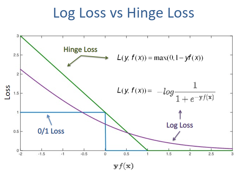
The loss function that helps maximize the margin is hinge loss:
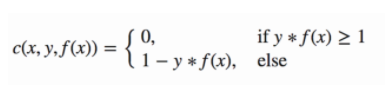
where y is class label +1 or -1, and $f(\mathbf{x}) = \mathbf{w}\mathbf{x}$ is predicted value. For example, If a classification is correct $\mathbf{w}\mathbf{x} \geq 1$ for label $\mathbf{y}=1$, then $\mathbf{y}[\mathbf{w}\mathbf{x}] \geq 1$. In this case there is no error (i.e. loss = 0). ↑ $\mathbf{y}[\mathbf{w}\mathbf{x}]$ , ↑ true. If classification is wrong $\mathbf{w}\mathbf{x} < 1$ for label $\mathbf{y}=1$, then y[wx] < 1. In this case, ↓ $\mathbf{y}[\mathbf{w}\mathbf{x}]$, ↑ loss. Thus, we can represent hinge loss function as
\(\ell(\mathbf{w},\mathbf{x},\mathbf{y}) = max (0, 1-\mathbf{y}[\mathbf{w}\cdot \mathbf{x}])\)
Kernel
Kernels in machine learning can help to construct non-linear decision boundaries using linear classifiers.
Soft Margin Formulation
This idea is based on a simple premise: allow SVM to make a certain number of mistakes and keep margin as wide as possible so that other points can still be classified correctly. This can be done simply by modifying the objective of SVM.
\[\underset{\mathbf{w}}{min}\hspace{4mm} \frac{1}{2}||\mathbf{w}||^2 + C\sum_{i=1}^{n} \xi_{i}\\ such\;that\hspace{4mm}(\mathbf{w}\mathbf{x}_i)\mathbf{y}_i + \xi_{i} \geq 1,\; \xi_{i}\geq 0\hspace{4mm} \forall i\]$\sum_{i=1}^{n} \xi_{i}$ is # of mistakes. $\xi{i}$ is called slack variables. The value of $\xi_i$ is the distance of $\mathbf{x}_i$ from the corresponding class’s margin if $\mathbf{x}_i$ is on the wrong side of the margin, otherwise zero. Thus the points that are far away from the margin on the wrong side would get more penalty. We want these $\xi{i}$ to be small. $C$ s a hyperparameter that decides the trade-off between maximizing the margin and minimizing the mistakes. When $C$ is small, we can tolerate more mistakes, and may introduce more bias that implies underfitting. And focus is more on maximazing the margin. Whereas, when $C$ is large, we can tolerate less mistakes, and may have less bias that implies overfitting. And focus is more on avoiding misclassification at the expense of keeping the margin small.
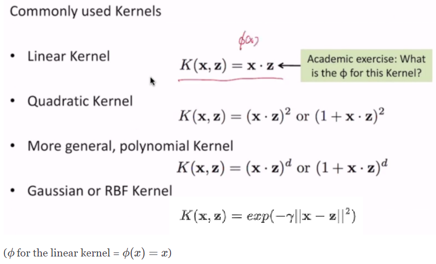
Kernel Tricks
Kernel functions are generalized functions that take the dot product of transformed input vectors $\phi(\mathbf{x})$ as input and output a score that denotes how similar the input vectors are. Kernel function has the capability of measuring similarity in higher dimensions , without increasing the computational costs too much. This is essentially known as the Kernel Trick.
A Kernel function can be written mathematically as follows:
\(K(\mathbf{x}, \mathbf{y}) = <\phi(\mathbf{x}), \phi(\mathbf{y})>\)
-
Gaussian/RBF Kernel
$\gamma$ sets the width of the bell shaped curve. ↑ $\gamma$ , narrower bell.
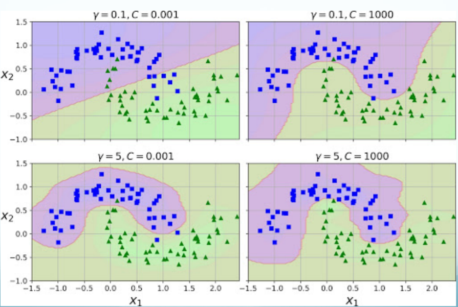
In conclusion,
↑ $\gamma$ , use similarity intensely, ↑ variance, overfitting.
↓ $\gamma$ , NOT use similarity intensely, ↑ bias, underfitting.
- RBF kernel is an inner product of two vectors in infinite dimensional space,
Decision Trees
reference1, reference2, reference3
Decision tree builds classification or regression models in the form of a tree structure. Decision trees can handle both categorical and numerical data.
ID3
The core algorithm for building decision trees called ID3, which is a top-down, greedy search through the space of possible branches with no backtracking. ID3 uses Entropy and Information Gain to construct a decision tree.
Information theory
- Entropy
Entropy is an information theory metric that measures the impurity or uncertainty in a group of observations. It determines how a decision tree chooses to split data. Consider a dataset with $c$ classes. The entropy may be calculated using the formula below:
\[E = -\sum_{i=1}^{c}p_ilog(p_i)\hspace{10mm}or\hspace{10mm}H(X)=-\sum_{x\in X}p(x)log(p(x))\]$p_i$ is the probability of randomly selecting an example in class $i$.
-
Conditional Entropy
conditional entropy quantifies the amount of information needed to describe the outcome of a random variable $Y$ given that the value of another random variable $X$ is known. The conditional entropy of $Y$ given $X$ is defined as
-
Information Gain (IG)
Information gain measures the reduction in entropy by splitting a dataset according to a given value of a random variable. Information gain helps us determine the quality of splitting. The more the entropy removed, the greater the information gain. The higher the information gain, the better the split. Maximizing information gain is equivalent to choosing features that minimize the conditional entropy. Because our feature choice doesn’t affect $H(Y)$, so it is really just an additive constant.
where $E_{parent}$ (before splitting) is the entropy of the parent node and $E_{children}$ (after splitting) is the average entropy of the child nodes. Let’s use an example to visualize information gain and its calculation.
Note: Very often greedy algorithms do NOT provide a globally optimum solution. Maximizing information gain node by node is greedy and not the same as optimizing over all possible tree configurations. Hence other trees with lower training error may exist.
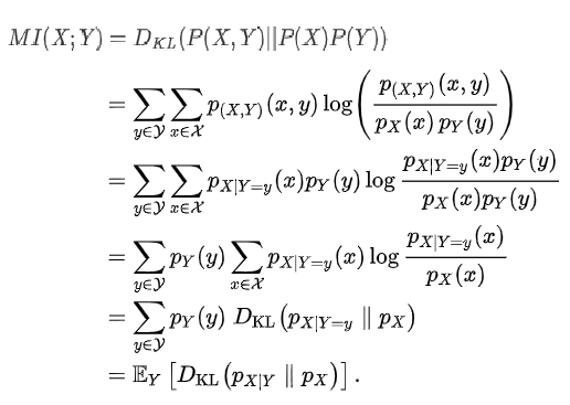
- Mutual Information
Mutual information is calculated between two variables and measures the reduction in uncertainty for one variable given a known value of the other variable.
Feature selection
Select the $K$ features that give us the most information about the label $Y$.
↓ $K$, ↑ bias, underfitting.$\hspace{5mm} \longleftarrow$ 0 depth trees (return most likely label) have no variance
↑ $K$, ↑ variance, overfitting.$\hspace{5mm}\longleftarrow$ Complete trees have no bias
Random Forests
Random Forest is a collection of trees with randomly selected features. It’s extremely robust to overfitting in practice. Individual tree learning (overfitting) matters much less. Drawback: doesn’t work well when only a few features are helpful.
↑ $#Trees$, ↑ prediction, ↑ slower, ↓ overfitting.
↓ $#Trees$, ↑ faster, ↑ overfitting.
Boosting
Boosting is an ensemble modeling technique that attempts to build a strong classifier from the number of weak classifiers. It is done by building a model by using weak models in series. Firstly, a model is built from the training data. Then the second model is built which tries to correct the errors present in the first model. This procedure is continued and models are added until either the complete training data set is predicted correctly or the maximum number of models are added.
AdaBoost
AdaBoost was the first really successful boosting algorithm developed for the purpose of binary classification. It is a very popular boosting technique that combines multiple “weak classifiers” into a single “strong classifier”. AdaBoost is very robust to overfitting.
What this algorithm does is that it builds a model and gives equal weights to all the data points. It then assigns higher weights to points that are wrongly classified. Now all the points which have higher weights are given more importance in the next model. It will keep training models until and unless a lowe error is received.
- First of all these data points will be assigned some weights. Initially, all the weights will be equal.
-
Calculate the Amount of Say/Importance/Influence and Total error to update the previous sample weights.
\[Total\;error = \frac{\#\;wrong\;output}{\#\;total\;samples}\]The Amount of Say/Performance of the stump will be:
\[\alpha_t=\frac{1}{2}ln(\frac{1-\varepsilon_t}{\varepsilon_t})\]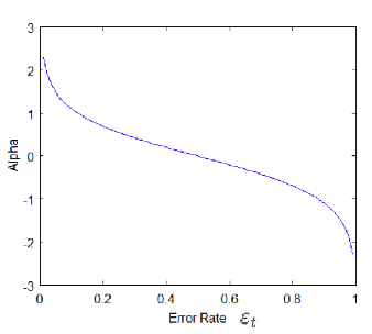
-
Update the weights. The wrong predictions will be given more weight whereas the correct predictions weights will be decreased.

The amount of say ($\alpha$) will be negative when the sample is correctly classified. The amount of say ($\alpha$) will be positive when the sample is miss-classified.
-
Normalize the new sample weights.
-
Output of the final hypothesis:
\[H(x)=sign(\sum_{t=1}^{T}\alpha_t h_t(x))\]where $\alpha_t$ is the Amount of Say and $h_t(x)$ is the actual label.